Acousto-optic beam steering for LiDARs

Li et al from U. Washington in Seattle published a paper titled "Frequency–angular resolving LiDAR using chip-scale acousto-optic beam steering"

Link: https://www.nature.com/articles/s41586-023-06201-6

Abstract:
Thanks to its superior imaging resolution and range, light detection and ranging (LiDAR) is fast becoming an indispensable optical perception technology for intelligent automation systems including autonomous vehicles and robotics. The development of next-generation LiDAR systems critically needs a non-mechanical beam-steering system that scans the laser beam in space. Various beam-steering technologies have been developed, including optical phased array, spatial light modulation, focal plane switch array, dispersive frequency comb and spectro-temporal modulation. However, many of these systems continue to be bulky, fragile and expensive. Here we report an on-chip, acousto-optic beam-steering technique that uses only a single gigahertz acoustic transducer to steer light beams into free space. Exploiting the physics of Brillouin scattering, in which beams steered at different angles are labelled with unique frequency shifts, this technique uses a single coherent receiver to resolve the angular position of an object in the frequency domain, and enables frequency–angular resolving LiDAR. We demonstrate a simple device construction, control system for beam steering and frequency domain detection scheme. The system achieves frequency-modulated continuous-wave ranging with an 18° field of view, 0.12° angular resolution and a ranging distance up to 115 m. The demonstration can be scaled up to an array realizing miniature, low-cost frequency–angular resolving LiDAR imaging systems with a wide two-dimensional field of view. This development represents a step towards the widespread use of LiDAR in automation, navigation and robotics. 

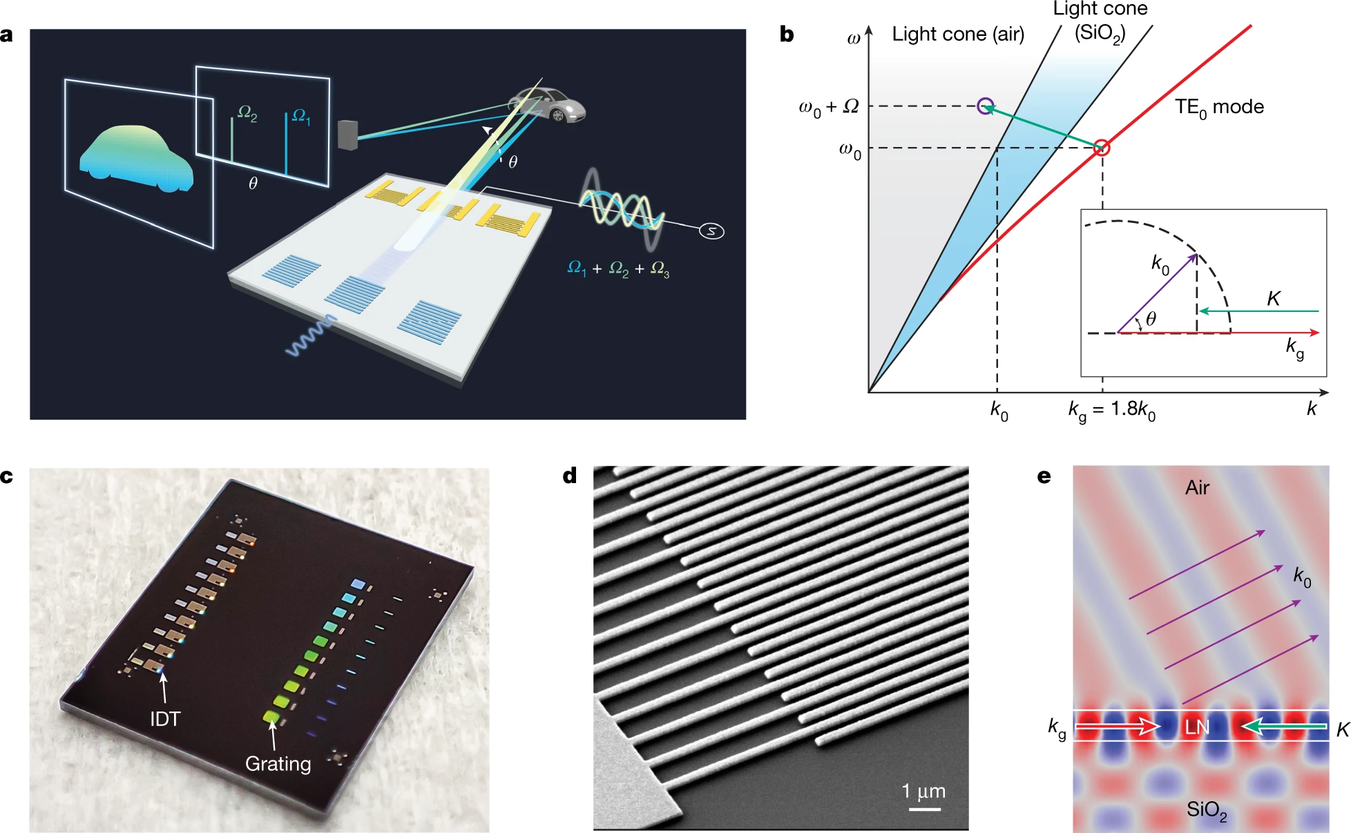
a, Schematic illustration of the FAR LiDAR scheme based on AOBS. b, Dispersion diagram of the acousto-optic Brillouin scattering process. The dispersion curve of the TE0 mode of the LN planar waveguide is simulated and plotted as the red curve. At frequency ω0 (wavelength 1.55 μm), the mode wavenumber is 1.8k0 (red circle). The counter-propagating acoustic wave (green arrow) scatters the light into the light cone of air (purple circle in the grey shaded area). For clarity, the frequency axis is not to the scale. Inset: momentum vector relation of the Brillion scattering. The light is scattered into space at an angle θ from the surface. c, Photograph of an LNOI chip with ten AOBS devices. d, Scanning electron microscope image of the IDT. The period is chirped from 1.45 to 1.75 μm. e, Finite-element simulation of the AOBS process showing that light is scattered into space at 30° from the surface.

a, Superimposed image of the focal plane when the beam is scanned across a FOV from 22° to 40°, showing 66 well-resolved spots. b, Magnified image of one spot at 38.8°. The beam angular divergence along kx is 0.11° (bottom inset) and along ky is 1.6° (left inset), owing to the rectangular AOBS aperture. c, Real-space image of light scattering from the AOBS aperture. The light intensity decays exponentially from the front of the IDT (x = 0), owing to the propagation loss of the acoustic wave. Fitting the integrated intensity along the x axis (bottom inset, yellow line) gives an acoustic propagation length of 0.6 ± 0.1 mm. d, The measured frequency–angle relation when the beam is steered by sweeping the acoustic frequency. a.u., arbitrary units. e–h, Dynamic multi-beam generation and arbitrary programming of 16 beams (e) at odd (f) and even (g) sites, and in a sequence of the American Standard Code for Information Interchange code of characters ‘WA’ (h).

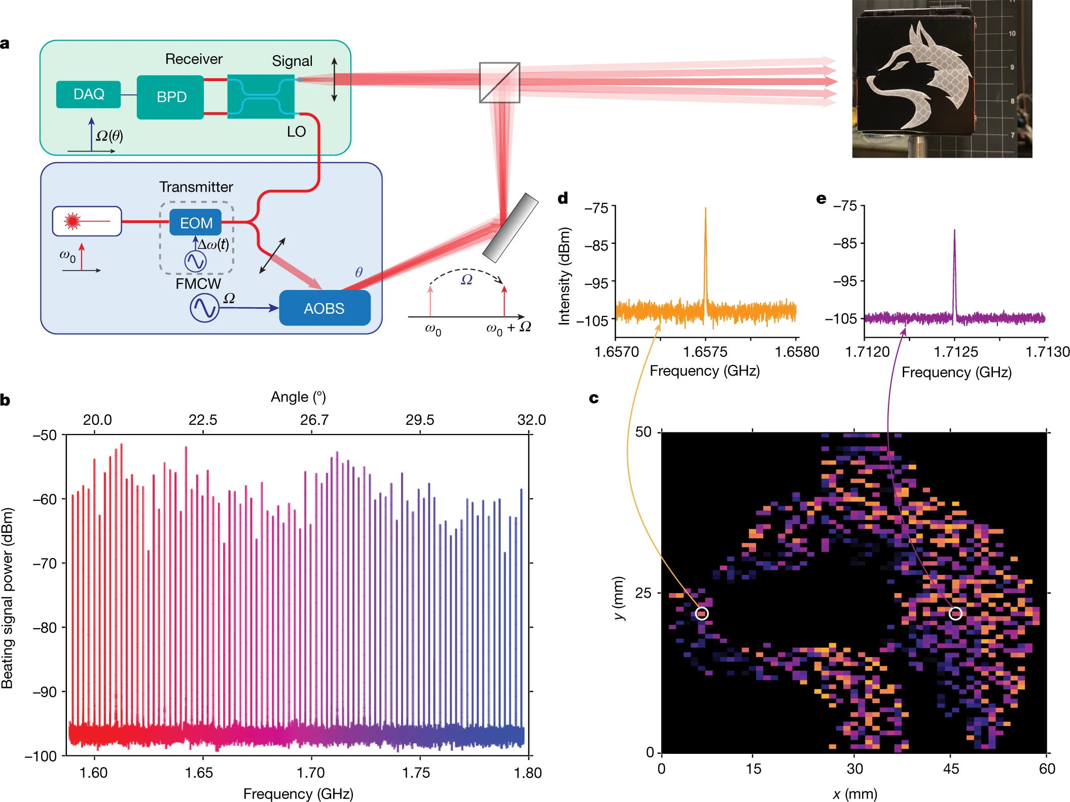
a, Schematics of the FAR LiDAR system. The transmitter includes a fixed-wavelength, fibre-coupled laser source, an EOM for FMCW (used in Fig. 4) and an AOBS device driven by a radio frequency source to steer the beam. An additional mirror is used to deflect the light towards the object. The coherent receiver uses homodyne detection to resolve the frequency shift of the reflected light by beating it with the LO, which is tapped from the laser source. A BPD is used to measure the beating signal, which is sampled by a digital data acquisition (DAQ) system or analysed by a real-time spectrum analyser. As a demonstration, a 60 × 50 mm cutout of a husky dog image made of retroreflective film is used as the object. It is placed 1.8 metres from the LiDAR system. b, Spectra of the beating signal at the receiver when the AOBS scans beam across the FOV. Using the measured frequency–angle relation in Fig. 2d, the beating frequency can be transformed to the angle of the object. c, FAR LiDAR image of the object. The position and brightness of each pixel are resolved from the beating frequency and power of the signal, respectively. d,e, The raw beating signal of two representative pixels (orange, d; purple, e).

 

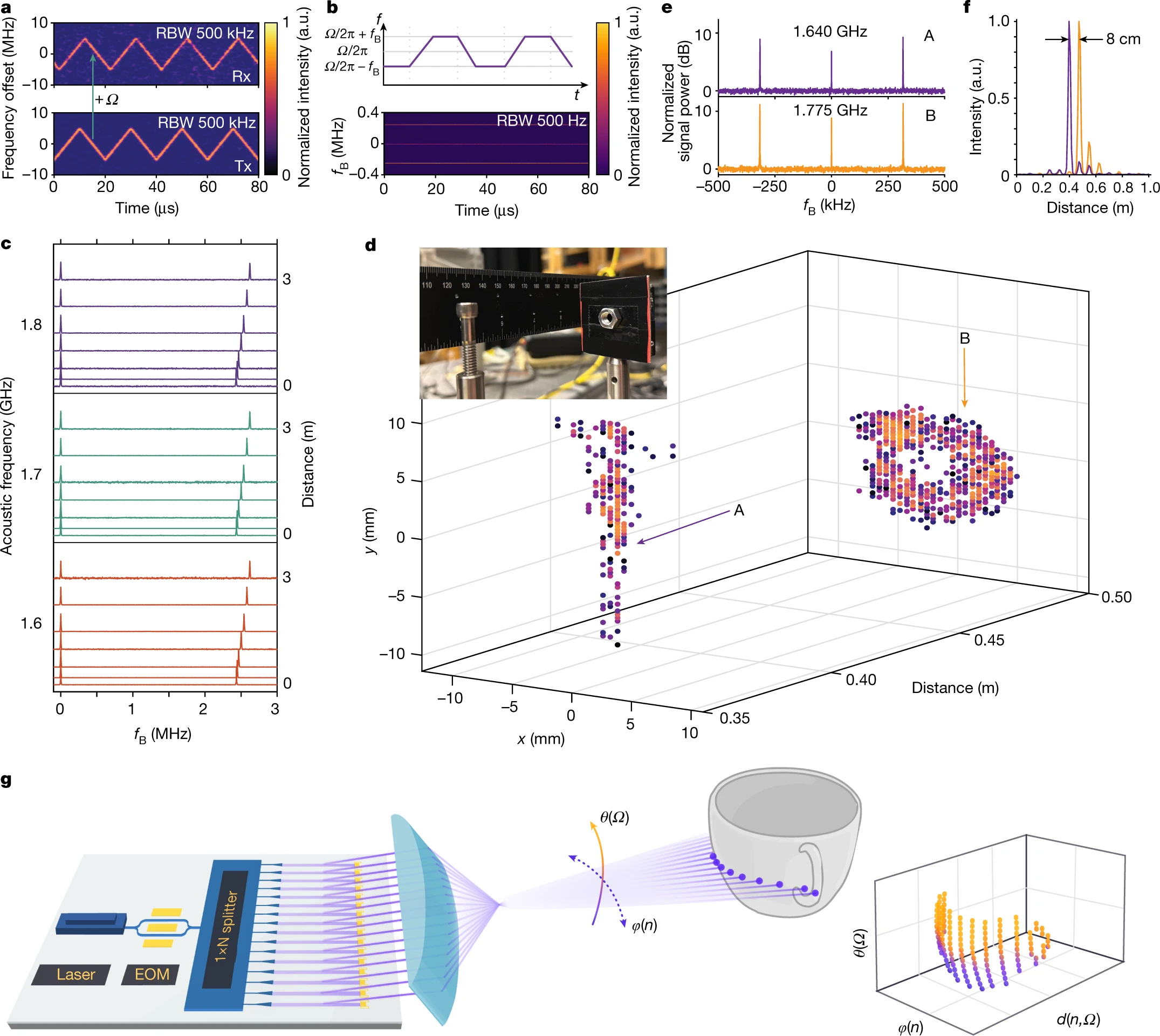
a, Time–frequency map of the transmitted light (bottom, Tx) and received light (top, Rx), both are chirped by a triangular waveform. The chirping rate is g = 1 MHz μs−1. The frequency of the received light is upshifted by the acoustic frequency Ω/2π (RBW, resolution bandwidth). a.u., arbitrary units. b, Top, schematic illustration of the frequency of the FMCW signal as a function of time. The frequency alternates between Ω/2π ± fB. Bottom, measured time–frequency map of the FMCW signal. Because of the upper sideband and the lower sideband) generated by the EOM, the FMCW frequencies at Ω/2π ± fB are present all the time. Also present is the frequency component at Ω/2π, which is from the unsuppressed optical carrier and used for FAR imaging. c, Spectra of FMCW signals when different acoustic frequencies (red, 1.6 GHz; green, 1.7 GHz; purple, 1.8 GHz) are used to steer the beam to reflectors placed at different angles and distances. d, 3D LiDAR image of a stainless steel bolt and a nut, placed 8.0 cm apart from each other, acquired by combining FAR and FMCW schemes. The FMCW chirping rate is g = 1 MHz μs−1 and frequency excursion fE = 1 GHz. Inset: photograph of the bolt and nut as the imaging objects. e, FMCW spectra of two representative points (A and B) in d, showing signals at Ω/2π (offset to zero frequency) and Ω/2π ± fB (offset to ±fB). f, Zoomed-in view of the FMCW signals at fB for point A and B. g, Our vision of a monolithic, multi-element AOBS system for 2D scanning, which, with a coherent receiver array (not shown), can realize 2D LiDAR imaging.